A review of four Machine Learning algorithms for classification
K-Nearest Neighbors, Decision Thee, Logistic Regression, and Support Vector Machines. How to choose the right algorithm? What to consider?
When choosing the correct algorithm, there is no short or straightforward answer. It always starts with what kind of problem you are trying to solve and what type of output you need. Which algorithm will give me a high accuracy? Well, it depends. There are several factors to consider when choosing the algorithm, such as type, size, shape, and dimensionality of the data, the learning time, interpretability, susceptibility to noise and overfitting, etc.
This article will review four machine learning algorithms for classification K-Nearest Neighbor, Decision Thee, Logistic regression, and Support Vector Machines. I will not explain in detail how these algorithms works, nor the math behind them; I will write a short paragraph about the algorithm and the data for which is suitable. Then I discuss the advantages and disadvantages with a focus on factors to consider when choosing the algorithm. At the end of the article, I created a table to summarize the discussion.
K- Nearest Neighbors (KNN)
K- Nearest Neighbors is one of the simplest machine learning algorithms. It is a non-parametric and lazy learner. KNN classifies a data point based on how its neighbors are classified. K is a number that specifies the number of nearest neighbors to include in the voting process. The reasoning is that the close points are likely to belong to the same class. Different metrics can be used to calculate the distance and find nearest neighbors; commonly used is Euclidean distance.
Advantages and disadvantages
The first advantage I will mention is based on the fact that it is a non-parametric algorithm, which means that it does not make assumptions/requires a specific distribution of the data. KNN is also straightforward to implement. When it comes to learning time, the KNN is very fast because it is a lazy learning algorithm; There is no clear training process involved. The training in KNN is simply a supply with instances where classes are known. Also, the advantage is that it has a few hyper-parameters to tune. So we have to decide only which distance to use and k- the number of neighbors to include in the voting process. When choosing the k number, it is important to avoid ties, so an odd number is used. Also, the number must not be multiple of the number of classes. It seems to be a rule of thumb to use the square root of the total number of data points in the training set.
One of the algorithm’s main disadvantages is a computationally costly testing time; it is needed to compute the distance to all known points. That is challenging in large datasets with a large number of features. There is also a Curse of Dimensionality problem, which describes that in the higher dimensions, points that may be different may appear close to each order; All the distances are more or less equal.
Further, the accuracy can be affected since KNN is sensitive to the frequency of the classes. For instance, if a particular class occurs more often in the training data, it will dominate the voting process.
KNN can also be sensitive to noise or irrelevant features. In particular, if we have a large dataset and small K, for example, K=3, and two of those are noise points. This could be enough to override the correct data points in the voting process in some regions, leading to poor performance on the test data, i.e., overfitting.
Logistic Regression
Logistic regression is used preferably for binary classification; the new observation can fall into one of two categories. However, it can also perform a multiclass classification. The analysis returns the probability that new data belongs to a particular category. Logistic regression assumes linearity in the data. Although it does not require the linear relationship between the dependent and independent variables, we estimate the probability for any given linear combination of the independent variables. It requires that the independent variables are linearly related to the log odds.
Advantages and disadvantages
In general, logistic regression is less prone to overfitting, the training of the model does not require high computation power, and it is fast at classifying new records. Besides, it is flexible for independent variables; it can handle categorical or continuous, or both. One of the main advantages is that it gives a highly interpretable result. Models parameters do not only indicate how relevant a feature is but also the direction of the relationship.
The disadvantage of the algorithm is that it cannot deal with non-linearly separable data nor multicollinearity. Also, only important and relevant features should be used to build a model; otherwise, it negatively affects the accuracy. Besides, this algorithm is sensitive to outliers, and it tends to overfit in high dimensional.
Decision Tree
A decision tree is a non-parametric algorithm, and the intuition behind it is straightforward. The algorithm predicts classes or values learning decision rules from the data features by traveling from a tree’s root node to a leaf. The tree builds recursively by splitting the nodes. The methods to determine when to split any further are based on finding a feature with the highest information gain. Internal nodes are split if the split makes it easier to distinguish between classes. The goal is with any further split, the data to get purer.
Advantages and disadvantages
Since it is a non-parametric model, no assumptions are made about the shape of data. It also works with numerical and categorical data. Additionally, one of the advantages is that the decision trees are highly interpreted and can be visually represented. Features without influence do not impact the results due to the decision-tree algorithm’s feature-selection ability. Also, the features that depend on each other do not affect the model.
However, the trees grow incrementally and thus cannot guarantee to return the globally optimal decision tree. The decision tree tends to overfit. It captures too much information about training data, and when the model is used to predict new data, the prediction would not be accurate. That is due to the model captured the noise from the training data. Hence the decision tree algorithms are sensitive to noise. Also, they are prone to becoming biased to the classes with a majority in the dataset.
Moreover, on the downside, pruning for the decision tree is not a straightforward process. Among many parameters that need to be tuned to avoid overfitting are the tree’s maximal depth, minimum samples required to be a leaf node, or impurity decrease parameter. The latest allows further growth of the tree (node splitting) if that induces a decrease of the impurity greater than or equal to the specified value.
The model can also overgrow and introduce complexity when dealing with high-dimensional datasets. When it comes to learning time, in such cases, it can require much computation. On the other hand, the trees are fast at classifying new records.
Support Vector Machines (SVM)
SVM assumes linear separability. The algorithm tends to find the optimum hyperplane to separate the space into classes. When the data is not linearly separable, it increases dimensionality to get linearly separable data using a kernel function. The kernel is essentially a mapping function, and it performs all calculations without leaving the original space, also known as the kernel trick.
Advantages and disadvantages
SVM can handle not frequently distributed data or data with unknown distribution. Also, the algorithm is not easily affected by noise since it depends on the support vectors only. A minor change to the data does not significantly affect the hyperplane. It has a good performance in high-dimensional spaces. SVM can be computationally heavy thus has a long training time on large datasets. On the other hand, since it uses only a subset of data points (support vectors) for decision-making, it quickly classifies new data points. Also, it has high accuracy, and it performs well in high dimensional spaces.
One of the limitations is the optimal design for a multiclass SVM classifier. The techniques used are One-vs.-one and one-vs.-rest. Multiclass SVMs dived the problem into multiple binary subproblems that are subsequently combined. Also, on the downside, the SVM does not have the interpretable models’ parameters. It is considered that this is a trade-off between the interpretability and accuracy of a model. Also, the algorithm has several hyperparameters that need to be tuned to achieve good results, such as kernel function, gamma, C(regularization parameter).

Conclusion
It is all about the dataset. So, always know your data. This is the first step when deciding which algorithm to use. When you know the type, size, and characteristics of data, it will help you narrow the selection. Then you can try out a couple of different algorithms, do hyperparameters tuning, and compare them based on the performance measures. The real question is which algorithm fits best for my data.